Geometry and Kinematics

Build a graphene momentum path and first-zone mesh. Then inspect inner-potential dispersion, detector-frame polarization, and a geometry Jacobian.

import jax
import jax.numpy as jnp
import matplotlib.pyplot as plt

from diffpes.simul import (
    kz_from_inner_potential,
    polarization_from_angles,
    polarization_to_spherical,
    rotate_polarization_grid,
)
from diffpes.tightb import (
    build_bz_mesh,
    build_kpath,
    kpath_arc_length,
    kpoints_frac_to_cart,
)
from diffpes.types import make_crystal_geometry, make_experiment_geometry

Build the Crystal and Experiment

Use real-space lattice vectors as matrix rows. The factory derives the reciprocal rows and expands no hidden coordinate convention. The long third vector makes the reciprocal z spacing small. Use a larger static shell to prove completeness.

a = 2.46
c = 20.0
lattice = jnp.array(
    [
        [a, 0.0, 0.0],
        [-0.5 * a, 0.5 * jnp.sqrt(3.0) * a, 0.0],
        [0.0, 0.0, c],
    ]
)
positions = jnp.array([[0.0, 0.0, 0.0], [1.0 / 3.0, 2.0 / 3.0, 0.0]])
crystal = make_crystal_geometry(lattice, positions, ("C", "C"))
polarization = polarization_from_angles(0.75, 0.0, "p")
experiment = make_experiment_geometry(50.0, polarization, inner_potential_ev=12.0)
print(crystal.reciprocal)
print(jnp.linalg.norm(experiment.polarization))

[[ 2.55414037  1.47463363 -0.        ]
 [ 0.          2.94926726  0.        ]
 [ 0.         -0.          0.31415927]]
1.0

Plot a Path and Zone Mesh

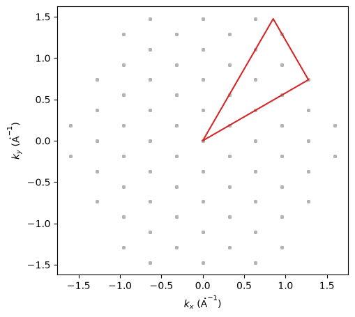
The path builder returns fractional coordinates. Convert them before any Cartesian distance, angle, or direction calculation.

anchors = jnp.array(
    [
        [0.0, 0.0, 0.0],
        [1.0 / 3.0, 1.0 / 3.0, 0.0],
        [0.5, 0.0, 0.0],
        [0.0, 0.0, 0.0],
    ]
)
path = build_kpath(anchors, crystal, 41, ("Gamma", "K", "M", "Gamma"))
distance = kpath_arc_length(path, crystal)
path_cartesian = kpoints_frac_to_cart(path.kpoints, crystal)
grid, first_zone = build_bz_mesh(crystal, 17, shell_radius=11)
grid_cartesian = kpoints_frac_to_cart(grid.kpoints, crystal)

fig, ax = plt.subplots(figsize=(6, 5))
ax.scatter(
    grid_cartesian[first_zone, 0],
    grid_cartesian[first_zone, 1],
    s=6,
    color="0.7",
)
ax.plot(path_cartesian[:, 0], path_cartesian[:, 1], color="tab:red")
ax.set_xlabel(r"$k_x$ ($\mathrm{\mathring{A}}^{-1}$)")
ax.set_ylabel(r"$k_y$ ($\mathrm{\mathring{A}}^{-1}$)")
ax.set_aspect("equal")
plt.show()

Plot Inner-Potential Dispersion

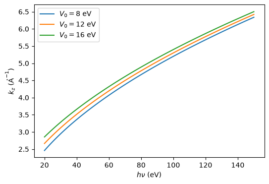
Vary \(V_0\) at fixed parallel momentum. The result remains inside the JAX graph for inversion and experiment design.

photon_energy = jnp.linspace(20.0, 150.0, 100)
k_parallel = jnp.asarray(0.5)
inner_potentials = jnp.asarray([8.0, 12.0, 16.0])

def kz_curve(inner_potential):
    return jax.vmap(
        lambda energy: jnp.real(
            kz_from_inner_potential(
                energy,
                experiment.work_function_ev,
                inner_potential,
                k_parallel,
            )[0]
        )
    )(photon_energy)

kz_curves = jax.vmap(kz_curve)(inner_potentials)
fig, ax = plt.subplots(figsize=(6, 4))
for inner_potential, values in zip(inner_potentials, kz_curves, strict=True):
    ax.plot(photon_energy, values, label=rf"$V_0={float(inner_potential):.0f}$ eV")
ax.set_xlabel(r"$h\nu$ (eV)")
ax.set_ylabel(r"$k_z$ ($\mathrm{\mathring{A}}^{-1}$)")
ax.legend()
plt.show()

Rotate the Polarization

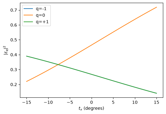
Rotate one p-polarized amplitude across the horizontal slit. The spherical weights show how the detector frame redistributes its components.

tx = jnp.deg2rad(jnp.linspace(-15.0, 15.0, 61))
ty = jnp.asarray([0.0])
rotated = rotate_polarization_grid(experiment.polarization, tx, ty, "H")
spherical = jax.vmap(polarization_to_spherical)(rotated[:, 0, :])
weights = jnp.abs(spherical) ** 2

fig, ax = plt.subplots(figsize=(6, 4))
for index, label in enumerate(("q=-1", "q=0", "q=+1")):
    ax.plot(jnp.rad2deg(tx), weights[:, index], label=label)
ax.set_xlabel(r"$t_x$ (degrees)")
ax.set_ylabel(r"$|\epsilon_q|^2$")
ax.legend()
plt.show()

Build the Geometry Jacobian

Differentiate one photon-energy scan with respect to \(V_0\), \(W\), and every photon-energy point. This Jacobian supplies the geometry information block.

scan_energy = jnp.linspace(25.0, 100.0, 8)

def scan(parameters):
    inner_potential = parameters[0]
    work_function = parameters[1]
    energies = parameters[2:]
    values, _ = jax.vmap(
        lambda energy: kz_from_inner_potential(
            energy,
            work_function,
            inner_potential,
            k_parallel,
        )
    )(energies)
    return jnp.real(values)

parameters = jnp.concatenate(
    (
        jnp.stack(
            (experiment.inner_potential_ev, experiment.work_function_ev)
        ),
        scan_energy,
    )
)
jacobian = jax.jacfwd(scan)(parameters)
print(jacobian.shape)
print(jacobian[:, 0])

(8, 10)
[0.04524925 0.03917244 0.03502908 0.03197228 0.02959744 0.02768367
 0.0260988  0.02475827]

Every printed \(V_0\) derivative is positive for these propagating channels. The geometry guide explains the validity domain and the \(W\leftrightarrow E_F\) gauge.