Quickstart: From Bands to a Differentiable ARPES Spectrum

Build a synthetic band structure and attach orbital characters. Then simulate two ARPES fidelity levels and differentiate the complete spectrometer model with jax.grad. The example runs on a CPU in less than one minute. The documentation build executes each code cell and displays its output.

Installation

Install diffpes from PyPI:

pip install diffpes

The diffpes import enables 64-bit precision in JAX. It also configures multithreaded CPU execution. You do not need to set jax_enable_x64. Verify the configuration:

import diffpes
import jax
import jax.numpy as jnp
import matplotlib.pyplot as plt

print(f"diffpes {diffpes.__version__}")
print(f"x64 enabled: {jax.config.jax_enable_x64}")

diffpes 2026.6.4
x64 enabled: True

A Synthetic Band Structure

diffpes usually consumes electronic-structure output from DFT codes. diffpes.inout parses VASP EIGENVAL and PROCAR files. The simulation layer also accepts plain arrays. Start with two cosine bands on a one-dimensional k-path. They represent nearest-neighbor tight binding on a chain.

The eigenvalue array has shape [nkpt, nband]. The first axis indexes points along the momentum path. The second axis indexes bands. The array stores energies in eV relative to the Fermi level at ef = 0.0. A small phase offset removes the symmetry relation between the bands. This offset makes later matrix-element effects easier to identify.

nkpt = 200
nband = 2
kpath = jnp.linspace(-jnp.pi, jnp.pi, nkpt)
band_lower = -1.2 - 0.8 * jnp.cos(kpath)
band_upper = -0.4 - 0.9 * jnp.cos(kpath + 0.3)
eigenbands = jnp.stack([band_lower, band_upper], axis=1)
print(f"eigenbands shape: {eigenbands.shape}")

eigenbands shape: (200, 2)

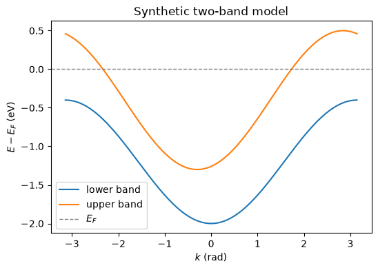
Plot the two dispersions. The upper band crosses the Fermi level near the zone boundary. Fermi-Dirac occupation therefore suppresses part of it in the simulated spectrum.

fig, ax = plt.subplots(figsize=(6, 4))
ax.plot(kpath, eigenbands[:, 0], label="lower band")
ax.plot(kpath, eigenbands[:, 1], label="upper band")
ax.axhline(0.0, color="gray", linestyle="--", linewidth=1, label=r"$E_F$")
ax.set_xlabel(r"$k$ (rad)")
ax.set_ylabel(r"$E - E_F$ (eV)")
ax.set_title("Synthetic two-band model")
ax.legend()
plt.show()

Orbital Weights

The band structure alone does not determine ARPES intensity. Each state’s orbital character controls its photoemission strength for a photon energy and polarization. diffpes stores this character in an orbital-projection array with shape [nkpt, nband, natom, 9]. This shape matches the VASP PROCAR layout.

The last axis follows the VASP 9-orbital ordering, zero-based:

Index	0	1	2	3	4	5	6	7	8
Orbital	\(s\)	\(p_y\)	\(p_z\)	\(p_x\)	\(d_{xy}\)	\(d_{yz}\)	\(d_{z^2}\)	\(d_{xz}\)	\(d_{x^2-y^2}\)

weights[:, 0, 0, 2] contains the \(p_z\) weight for band 0 and atom 0 at each k-point. Build a one-atom model. The lower band changes smoothly from \(p_z\) at the zone center to \(p_x\) at the zone boundary. The upper band uses a fixed 70/30 mixture of \(d_{xy}\) and \(d_{x^2-y^2}\).

natom = 1
weights = jnp.zeros((nkpt, nband, natom, 9))
pz_weight = jnp.cos(kpath / 2.0) ** 2
px_weight = jnp.sin(kpath / 2.0) ** 2
weights = weights.at[:, 0, 0, 2].set(pz_weight)
weights = weights.at[:, 0, 0, 3].set(px_weight)
weights = weights.at[:, 1, 0, 4].set(0.7)
weights = weights.at[:, 1, 0, 8].set(0.3)
surface_orb = weights
print(f"surface_orb shape: {surface_orb.shape}")

surface_orb shape: (200, 2, 1, 9)

Simulating the Spectrum

The diffpes.simul.simulate_expanded() entry point accepts plain arrays and scalar experiment parameters. It selects one of six fidelity levels: novice, basic, basicplus, advanced, expert, or soc. Each level adds physics. The guides describe all levels.

Start with level="basic". This level applies Gaussian broadening with sigma in eV. It applies Fermi-Dirac occupation at the specified temperature. It also applies heuristic orbital weights that depend on photon_energy. Use 21.2 eV, the He-I\(\alpha\) line of a helium lamp.

spectrum_basic = diffpes.simul.simulate_expanded(
    level="basic",
    eigenbands=eigenbands,
    surface_orb=surface_orb,
    ef=0.0,
    sigma=0.06,
    fidelity=2000,
    temperature=30.0,
    photon_energy=21.2,
)
print(f"intensity shape: {spectrum_basic.intensity.shape}")
print(f"energy axis shape: {spectrum_basic.energy_axis.shape}")

intensity shape: (200, 2000)
energy axis shape: (2000,)

The result is an ArpesSpectrum PyTree with two fields. Its intensity field has shape [nkpt, fidelity] and contains the photoemission map \(I(k, E)\). Its energy_axis field has shape [fidelity]. The axis extends 1 eV beyond each band-energy limit.

Now simulate the same system at level="advanced". This level replaces the heuristic weights with interpolated Yeh-Lindau photoionization cross-sections. It also adds polarization-dependent selection rules. The factor \(|\hat{\varepsilon} \cdot \vec{d}\,|^2\) weights each orbital channel. Here, \(\hat{\varepsilon}\) is the electric-field direction. Select p-polarized light with "LHP", which means linear horizontal polarization. Set its incident angle to 45 degrees. Other tokens are "LVP", "RCP", "LCP", "LAP", and "unpolarized".

spectrum_adv = diffpes.simul.simulate_expanded(
    level="advanced",
    eigenbands=eigenbands,
    surface_orb=surface_orb,
    ef=0.0,
    sigma=0.06,
    fidelity=2000,
    temperature=30.0,
    photon_energy=21.2,
    polarization="LHP",
    incident_theta=45.0,
)
print(f"intensity shape: {spectrum_adv.intensity.shape}")

intensity shape: (200, 2000)

Plot both spectra side by side. Transpose the intensity array so that energy uses the vertical detector axis.

energy_axis = spectrum_basic.energy_axis
extent = [
    float(kpath[0]),
    float(kpath[-1]),
    float(energy_axis[0]),
    float(energy_axis[-1]),
]
fig, axes = plt.subplots(1, 2, figsize=(10, 4), sharey=True)
titles = ["basic: heuristic weights", "advanced: p-pol matrix elements"]
for ax, spec, title in zip(axes, [spectrum_basic, spectrum_adv], titles):
    ax.imshow(
        spec.intensity.T,
        origin="lower",
        aspect="auto",
        extent=extent,
        cmap="inferno",
    )
    ax.set_title(title)
    ax.set_xlabel(r"$k$ (rad)")
axes[0].set_ylabel(r"$E - E_F$ (eV)")
axes[0].set_ylim(-2.5, 0.5)
plt.show()

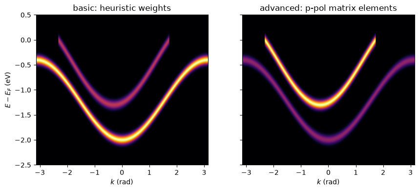
Both panels have the same band positions. Matrix elements rescale peaks but do not move them. The levels change the relative brightness within and between the bands. In the basic spectrum, the intensity follows the total orbital weight. The lower band is therefore approximately uniform. In the advanced spectrum, the \(p_z \to p_x\) change couples differently to the p-polarized field. This coupling changes the brightness along \(k\). The \(d\)-derived upper band also receives a different cross-section scale. Experiments can confuse this intensity variation with a change in the electronic structure. A matrix-element forward model separates these effects. The Fermi-Dirac factor also suppresses both bands above \(E_F\).

The Differentiable Hook

Pure JAX operations implement the broadening, occupation, cross-sections, and polarization weights. The complete spectrometer model is therefore differentiable. Define a scalar observable to demonstrate this property. The observable is the total intensity in a narrow window below the Fermi level. Its variables are the resolution sigma and the Fermi energy ef.

def window_intensity(sigma, ef):
    spec = diffpes.simul.simulate_expanded(
        level="basic",
        eigenbands=eigenbands,
        surface_orb=surface_orb,
        ef=ef,
        sigma=sigma,
        fidelity=2000,
        temperature=30.0,
        photon_energy=21.2,
    )
    in_window = (spec.energy_axis > -0.3) & (spec.energy_axis < 0.0)
    return jnp.sum(spec.intensity * in_window)

Use jax.grad to differentiate this scalar with respect to either argument. The derivative includes the lineshape, Fermi function, and orbital weighting.

grad_sigma = jax.grad(window_intensity, argnums=0)(0.06, 0.0)
grad_ef = jax.grad(window_intensity, argnums=1)(0.06, 0.0)
print(f"d(window intensity)/d(sigma) = {float(grad_sigma):.1f} per eV")
print(f"d(window intensity)/d(ef)    = {float(grad_ef):.1f} per eV")

d(window intensity)/d(sigma) = 31632.8 per eV
d(window intensity)/d(ef)    = 6596.9 per eV

Both gradients are positive. Broadening moves spectral weight from the band bottoms into the window near \(E_F\). A higher Fermi level increases the occupied part of the upper band in the window. JAX computes exact derivatives instead of finite differences.

Differentiability makes the spectrometer model invertible. Apply jax.grad to a chi-squared difference between simulated and measured spectra. The Equinox and Optimistix stack can then recover band parameters, self-energies, or experimental settings from data. The gradients can also quantify how a 10 meV improvement in resolution changes the measurement. This calculation does not require a parameter sweep.

Next Steps

• Theory and architecture guides: Read about the six fidelity levels and their dipole physics. Check support for the grad, jit, and vmap transformations.

• API reference: Read the complete function documentation. Use the diffpes.inout VASP readers with real DFT output.